Imagine flipping a coin and getting 10 heads in a row. You might wonder. How about 15? Something is definitely up, right?
So when a team goes on an extended winning streak, my gut tells me that something so unlikely is happening that it proves sports contests must be more than just (weighted) coin flips.
But is that true? To convince myself, I work out the probabilities of winning streaks of different lengths, where games are modeled as weighted coin flips, occurring during a single season. I use each team’s actual winning percentage during one season (here 2018) as the weight. I then compare those odds to the actual lengths of winning streaks that occured during that season.
I admit, what I find is a little surprising.
Python packages
We start by importing some standard Python packages:
from __future__ import division
import os
import numpy as np
import pandas as pd
import sys
import matplotlib.pyplot as plt
from matplotlib.pyplot import figure
import seaborn

%matplotlib inline
plt.style.use('ggplot')

sys.setrecursionlimit(20000)
Next, since we want to know how unlikely are long winning streaks, we need to estimate what those odds are in theory, from simple statistics.
We model the odds of any one win as a weighted coin flip, where the weight is simply the team’s winning percentage.
Here I’ll use a recursive algorithm to estimate the probability of a streak of length winStreak during a season numGames long, for a team whose season-long record is winPercent.
Naturally, we expect the probability to increase for:
- shorter streaks
- better teams
- longer seasons
def probability_of_streak(numGames, winStreak, winPercent, saved = None):

        if saved == None: saved = {}

        ID = (numGames, winStreak, winPercent)

        if ID in saved: return saved[ID]
        else:
            if winStreak > numGames or numGames <=0:
                result = 0
            else:
                result = winPercent**winStreak
                for firstWin in xrange(1, winStreak+1):
                    pr = probability_of_streak(numGames-firstWin, winStreak, winPercent, saved)
                    result += (winPercent**(firstWin-1))*(1-winPercent)*pr

        saved[ID] = result

        return result
Define a function splits the season into arrays representing winning streaks.
def consecutive(data, stepsize=0):
    # define an empty array the length of a season and replace 0 with 1 for each Win.
    sched = np.zeros(np.size(data))
    sched[np.isin(data,'W')] = 1
    # split into chunks of winning streaks
    return np.split(sched, np.where(np.diff(sched) != stepsize)[0]+1)
Define a function to group streaks by wins and losses.
def group_streaks(sched):
    all_streaks = consecutive(sched)
    longest_streak = np.size(max(all_streaks,key=len))
    wins = np.zeros(longest_streak,dtype=np.int)
    loss = np.zeros(longest_streak, dtype=np.int)
    for i in all_streaks:
        ind = np.size(i)-1
        if i[0] == 1:
            wins[ind] += 1
        else:
            loss[ind] += 1

    return [wins, loss]
def winning_percentage(streaks):
    wp = {}
    gp = {}
    for team in streaks:
        total_number_games = np.sum((np.arange(np.size(streaks[team][0]))+1) * streaks[team][0]) + np.sum((np.arange(np.size(streaks[team][1]))+1) * streaks[team][1])
        gp[team] = total_number_games
        wp[team] = np.sum((np.arange(np.size(streaks[team][0]))+1) * streaks[team][0]) / total_number_games
    return wp,gp
Download Data
The following files were grabbed from Baseball Reference. I store them in directories categorized by year, as well as Al and NL.
path_files = '/data/baseball/Baseball-Reference/schedule_results/2018/'
leagues    = ['AL','NL']
We loop through each Leage and Team, storing Wins and Losses as W and L in a Pandas Dataframe. Additionally, we convert walk-off wins and losses (‘W-wo’, ‘L-wo’) to ‘W’ and ‘L’.
Lastly, we store streaks for each team in a streaks dictionary.
streaks = {}
for league in leagues:
    path_csv = path_files + league + '/'
    fnames = os.listdir(path_csv)
    for itm in fnames:
        team = itm.split('.')[0].split('_')[0]
        pd.read_csv(path_csv+itm)
        df = pd.read_csv(path_csv+itm)
        df['W/L'][df['W/L'] == 'W-wo'] = 'W'
        df['W/L'][df['W/L'] == 'L-wo'] = 'L'
        a = df['W/L'].values
        streaks[team] = group_streaks(a)
Lets look win streaks in the streaks dictionary. Beginning with 2 game win streaks, which are the most frequent, we see a rapid drop off, although more than half have had one long streak (greater than 5).
print('Team',str(np.arange(15)+2))
for t in streaks:
    print(t,str(streaks[t][0][1:]))
('Team', '[ 2  3  4  5  6  7  8  9 10 11 12 13 14 15 16]')
('NYY', '[14  4  5  1  0  0  1  1]')
('MIL', '[11  9  2  1  0  0  2]')
('MIN', '[7 4 4 2 1 0 0]')
('TOR', '[3 6 4 1]')
('ATL', '[11  5  2  3  2]')
('BOS', '[12  5  6  1  1  0  1  1  1]')
('DET', '[7 2 3 1 0 0 0 0 0 0]')
('CIN', '[10  4  0  0  1  1  0]')
('NYM', '[13  3  2  0  0  0  0  1]')
('BAL', '[5 2 1 0 0 0 0 0]')
('COL', '[7 5 4 2 1 1 1]')
('OAK', '[10  3  5  1  4]')
('TEX', '[11  3  1  0  0  1]')
('MIA', '[12  3  2  0  0]')
('SEA', '[8 4 4 2 0 0 1]')
('PIT', '[8 3 1 4 0 0 0 0 0 1]')
('CHC', '[14  4  3  2  1  1]')
('STL', '[14  5  2  2  0  0  1]')
('CLE', '[9 7 0 2 2 1]')
('CWS', '[10  4  2  0  0  0  0]')
('HOU', '[7 7 1 3 3 1 0 0 0 0 1]')
('SFG', '[8 6 4 1 0 0 0 0 0 0]')
('WAS', '[15  8  3  1  1  1]')
('PHI', '[10  4  2  1  2  0  0  0]')
('SDP', '[9 5 1 0 0 0]')
('LAD', '[9 8 7 2 0]')
('TBR', '[6 4 2 4 1 0 2]')
('LAA', '[9 4 5 0 1 1]')
('KCR', '[7 3 1 0 1 0 0 0 0]')
('ARI', '[10 10  2  1  0  0]')
Looks like a lot of long winning streaks. But how does that compare to what theory predicts?
To answer that, we count how many teams have had streaks greater than N, from N = 1 to 15.
streak_size = 15
win_percent, games_played = winning_percentage(streaks)
real_win_streaks  = np.zeros(streak_size)
cum_win_streaks  = np.zeros(streak_size)
win_predict = np.zeros(streak_size)
for t in streaks:
    x = (np.arange(np.size(streaks[t][0])))
    cumulative_wins = np.cumsum(streaks[t][0][::-1])[::-1]
    ind_non_zero = np.where(streaks[t][0] > 0)
    cind_non_zero = np.where(cumulative_wins > 0)
    real_win_streaks[x[ind_non_zero]] += 1
    cum_win_streaks[x[cind_non_zero]] += 1
    for p in np.arange(streak_size):
        win_predict[p] += probability_of_streak(games_played[t], p+1, win_percent[t])
Let’s plot win streak length W vs. the number of teams that reached that threshold; in theory and reality. We expect all thirty teams to have had 2 game streaks, most to have had 3 game streaks, fewer to have 4 game streaks, and so on; how they track after that is when it gets interesting: if I was right and baseball is nothing like flipping a coin, theory should drop much more quickly than reality.
figure(num=None, figsize=(8, 6), dpi=80, facecolor='w', edgecolor='k')
plt.step(np.arange(streak_size)+1,cum_win_streaks,linestyle = '--',label='Actual')
plt.step(np.arange(streak_size)+1,np.round(win_predict),label='Theory')
plt.legend()
plt.title('Number of Teams with Winning Streaks of Length W')
plt.xlabel('W - Winning Streak Length')
plt.ylabel('Number of Teams')
plt.show()
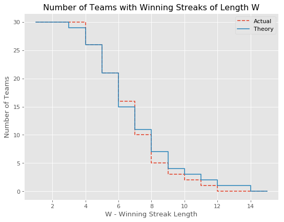
Instead, we find reality looks a lot like theory! Moreover, while we find a slight excess of teams with winning streaks of 4 or fewer, we find a much larger deficit of teams with winning streaks greater than 6. In fact no team has a winning streak of more than 12, where in theory there should have been closer to 3.
If anything, this contradicts my intuition that streaks are special — the lack of streaks is the actual surprise.
We can do the same for losing streaks.
streak_size = 15
lose_percent, games_played = winning_percentage(streaks)
real_lose_streaks  = np.zeros(streak_size)
cum_lose_streaks  = np.zeros(streak_size)
lose_predict = np.zeros(streak_size)
for t in streaks:
    x = (np.arange(np.size(streaks[t][1])))
    cumulative_losses = np.cumsum(streaks[t][1][::-1])[::-1]
    ind_non_zero = np.where(streaks[t][1] > 0)
    cind_non_zero = np.where(cumulative_losses > 0)
    real_lose_streaks[x[ind_non_zero]] += 1
    cum_lose_streaks[x[cind_non_zero]] += 1
    for p in np.arange(streak_size):
        lose_predict[p] += probability_of_streak(games_played[t], p+1, lose_percent[t])

figure(num=None, figsize=(8, 6), dpi=80, facecolor='w', edgecolor='k')
plt.step(np.arange(streak_size)+1,cum_lose_streaks,linestyle = '--',label='Actual')
plt.step(np.arange(streak_size)+1,lose_predict,label='Theory')
plt.legend()
plt.title('Number of Teams with Losing Streaks of Length L')
plt.xlabel('L - Losing Streak Length')
plt.ylabel('Number of Teams')
plt.show()
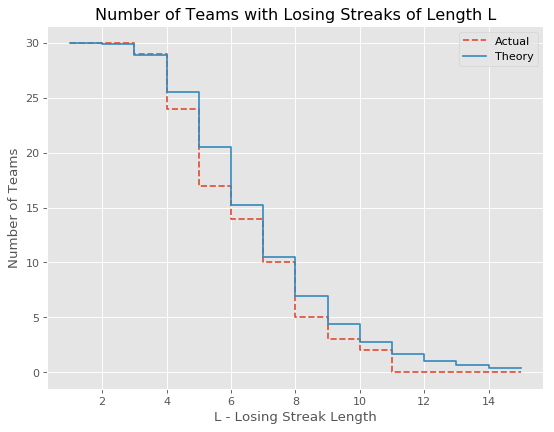
At last the human element presents itself. There are many fewer teams with losing streaks greater than 4 and above than predicted by the biniomal distribution alone. Lose a few games and you can be sure some changes will occur; this may be evidence that they work!