Ten hits in a single game can have very different results depending how they’re distributed — spread out they can be relatively harmless (unless they’re all home runs!), but clustered together and they can cause some serious damage. There is a general consensus that the distribution of hits comes down to luck, or clusterluck, but I can’t help but wonder if it’s possible to nudge lineups towards more clustering.
To begin to answer that I thought, why not use a simulation to compare the outcomes of the simplest possible scenarios: lineups with on-base percentages (OBPs) in ascending and descending orders?
Here I show each step of the simulation, which includes:
- drawing lineups of on-base percentages, drawn from a realistic distribution.
- estimating whether the batter makes an out using Bernoulli function, then
- simulating single games in the simplest way possible: 9 innings, 3 outs, on base moves everyone up one spot.
- simulating entire seasons 5000 times.
Python packages
We start by importing some standard Python packages:
from __future__ import absolute_import, division, print_function
import os
import numpy as np
import pandas as pd
import seaborn as sns
import scipy
from scipy.optimize import curve_fit
import sys
import scipy.stats as stats
from matplotlib.pyplot import figure
import matplotlib.pyplot as plt
plt.style.use('seaborn')
plt.tick_params(axis='x', colors='white')
plt.tick_params(axis='y', colors='white')
%matplotlib inline
Download Data
The following file containing batting data (Name, PA, HR, OBP, etc.) was grabbed from Fangraphs and stored locally.
We use Pandas to read the .csv file into a Dataframe named leaderboard.
path_leaderboard = '/data/baseball/Fangraphs/FanGraphs_Leaderboard_Full_2018.csv'
leaderboard = pd.read_csv(path_leaderboard)
Let’s see what leaderboard contains.
leaderboard_keys = [i for i in leaderboard]
print(leaderboard_keys)
leaderboard.head()
['Name', 'Team', 'G', 'PA', 'HR', 'R', 'RBI', 'SB', 'BB%', 'K%', 'ISO', 'BABIP', 'AVG', 'OBP', 'SLG', 'wOBA', 'wRC+', 'BsR', 'Off', 'Def', 'WAR', 'playerid']
| Name | Team | G | PA | HR | R | RBI | SB | BB% | K% | ... | AVG | OBP | SLG | wOBA | wRC+ | BsR | Off | Def | WAR | playerid | |
|---|---|---|---|---|---|---|---|---|---|---|---|---|---|---|---|---|---|---|---|---|---|
| 0 | Mookie Betts | Red Sox | 136 | 614 | 32 | 129 | 80 | 30 | 13.2 % | 14.8 % | ... | 0.346 | 0.438 | 0.640 | 0.449 | 185.0 | 6.9 | 69.1 | 11.6 | 10.4 | 13611 |
| 1 | Mike Trout | Angels | 140 | 608 | 39 | 101 | 79 | 24 | 20.1 % | 20.4 % | ... | 0.312 | 0.460 | 0.628 | 0.447 | 191.0 | 5.0 | 71.1 | 4.2 | 9.8 | 10155 |
| 2 | Jose Ramirez | Indians | 157 | 698 | 39 | 110 | 105 | 34 | 15.2 % | 11.5 % | ... | 0.270 | 0.387 | 0.552 | 0.391 | 146.0 | 12.0 | 50.6 | 4.6 | 8.0 | 13510 |
| 3 | Alex Bregman | Astros | 157 | 705 | 31 | 105 | 103 | 10 | 13.6 % | 12.1 % | ... | 0.286 | 0.394 | 0.532 | 0.396 | 157.0 | 3.4 | 51.4 | -0.6 | 7.6 | 17678 |
| 4 | Francisco Lindor | Indians | 158 | 745 | 38 | 129 | 92 | 25 | 9.4 % | 14.4 % | ... | 0.277 | 0.352 | 0.519 | 0.368 | 130.0 | 1.2 | 28.3 | 21.1 | 7.6 | 12916 |
5 rows × 22 columns
Define Simulation Functions
Next, we define the functions that get called by the simulations.
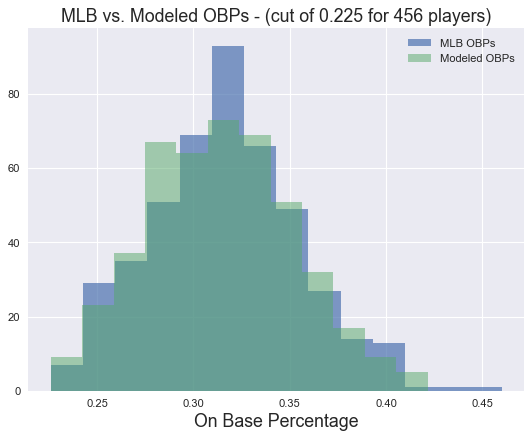
We begin by constructing a realistic distrubution of on-base percentages (OBPs), define_P, to draw from later. One way to do that is to simply fit a Gaussian to the OBPs found in leaderboard, i.e., the actual OPBs. Note, to make sure that the modeled lineup is not dominated by transient players, we define lower limits for OBP and minimum plate appearances (using stats.truncnorm) as 0.225 and 80, respectively.
def define_P(leaderboard, lower_obp = 0.225, min_plate_appearances = 80, year = 2018):
    n, bins = np.histogram(leaderboard.OBP[(leaderboard.PA > min_plate_appearances)], 'scott')
    bin_centres = (bins[:-1] + bins[1:])/2
    p0 = [1., 0., 1.]
    coeff, var_matrix = curve_fit(gauss, bin_centres, n, p0=p0)
    print('mean='+str(coeff[1]))
    print('std='+str(coeff[2]))
    upper = 1.0 # Can't reach base more than 100% percent of time
    X = stats.truncnorm(
        (lower_obp - coeff[1]) / coeff[2], (upper - coeff[1]) / coeff[2], loc=coeff[1], scale=coeff[2])
    return X, coeff
The function gauss is used to fit Gaussians to histograms.
def gauss(x, *p):
    A, mu, sigma = p
    return A*np.exp(-(x-mu)**2/(2.*sigma**2))
We then define draw_lineup to build a lineup by calling define_P, i.e., randomly drawing OBPs for 9 players.
def draw_lineup(P):
    lineup = {}
    lineup['OBP'] = P.rvs(9)
    return lineup
Check that our distribution of OBPs that we draw a lineup from looks correct.
For this simulation we’ll define
- Plate appearance lower limit (pa_cut) = 80
- OBP lower limit (lower_obp_cut) = 0.225
lower_obp_cut = 0.225
pa_cut = 80
test_OBP_Dist, test_coeff = define_P(leaderboard, lower_obp = lower_obp_cut, min_plate_appearances = pa_cut)
test_lineup  = draw_lineup(test_OBP_Dist)
Next we’ll confirm the real and modeled distributions look similar by overplotting their histograms.
mean_obp, sigma = test_coeff[1], test_coeff[2]
P = stats.truncnorm(
    (lower_obp_cut - mean_obp) / sigma, (1 - mean_obp) / sigma, loc=mean_obp, scale=sigma)
test_lineup_obp = P.rvs(np.size(leaderboard.OBP[(leaderboard.OBP > lower_obp_cut) & (leaderboard.PA > pa_cut)]))
plt.hist(leaderboard.OBP[(leaderboard.OBP > lower_obp_cut) & (leaderboard.PA > pa_cut)], 'scott', alpha = 0.70)
plt.hist(test_lineup_obp, 'scott' , alpha = 0.5)
plt.title("MLB vs. Modeled OBPs - (cut of "+str(lower_obp_cut)+" for "+str(len(test_lineup_obp))+" players)", fontsize=16)
plt.xlabel("On Base Percentage", fontsize=16)
labels= ["MLB OBPs","Modeled OBPs"]
plt.legend(labels)
The function bern_obp is used to decide, in each instance that it is called, whether the batter reaches base or not. For example, if obp is 0.500, then bern_obp will return 0 half the times that is it called, and 1 the other half.
def bern_obp(obp):
    ob = np.random.binomial(1, obp)
    return ob
The game_simulation function defined next is very basic: for 9 innings it steps through lineup and uses the Bernoulli function bern_obp to decide whether the batter is out or gets on base (effectively a base on ball). Once 3 outs are reached, the inning turns over.
Output is a dictionary innings which stores the box score of each inning. Next we’ll search them for streaks.
def game_simulation(lineup, game_length = 9):
    bases = np.zeros(3)
    innings = {}
    batter = 0
    runs   = 0
    for inning in np.arange(game_length)+1:
        #print 'inning ', str(inning)
        plays = []
        outs = 0
        while outs <3:
            play = bern_obp(lineup[batter])
            #print play
            if play == 0:
                outs+=1
            batter = batter+1
            if batter == 9:
                batter = 0
            plays.extend([play])

        innings[inning] = plays

    return innings
Count the streaks (or clusters) and cluster lengths found in innings dictionaries.
def on_base_streaks(innings, stepsize=0):
    cluster = []
    cluster_length = []
    for i in innings:
        streaks = np.split(innings[i], np.where(np.diff(innings[i]) != stepsize)[0]+1)
        for j in streaks:
            if (j[0] > 0) & (len(j) > 1):
                cluster.append(j)
                cluster_length.append(len(j))

    return cluster, cluster_length
Simple sum of total at-bats.
def count_number_at_bats(box_score):
    tot_at_bats = np.sum(np.sum(box_score.values()))
    return tot_at_bats
Simulate a full season by looping game_simulation 162 times.
Keep track of the box scores, number of streaks, and streak lengths in a dictionary named season_stats.
Note, we estimate every 5th game is only 8 innings long (non walk-off home win).
def team_season_simulation(lineup, season_length = 162):
    season_stats = {}
    season_stats['box'] = {}
    season_stats['streaks'] = {}
    season_stats['streak_lengths'] = {}
    # -- Estimate every 5th game is 8 innings --
    for g in np.arange(season_length)+1:
        if np.mod(g,5) == 0:
            game_length = 8
        else:
            game_length = 9

        season_stats['box'][g]     = game_simulation(lineup)
        season_stats['streaks'][g], season_stats['streak_lengths'][g]  = on_base_streaks(season_stats['box'][g])
    return season_stats
Game Simulation
nsims = 5000

td_streak_count = np.zeros(nsims)
bu_streak_count = np.zeros(nsims)
td_total_hits   = np.zeros(nsims)
bu_total_hits   = np.zeros(nsims)

obp_model, coeffs_model = define_P(leaderboard)

for i in np.arange(nsims):
    lineup = draw_lineup(obp_model)
    bottom_up = np.sort(lineup['OBP'])
    top_down  = np.sort(lineup['OBP'])[::-1]

    bu_sim = team_season_simulation(bottom_up)
    bu_streak_count[i] = sum([len(bu_sim['streak_lengths'][x]) for x in bu_sim['streak_lengths']])
    bu_total_hits[i]   = sum([count_number_at_bats(bu_sim['box'][x]) for x in bu_sim['streak_lengths']])
    td_sim = team_season_simulation(top_down)
    td_streak_count[i] = sum([len(td_sim['streak_lengths'][x]) for x in td_sim['streak_lengths']])
    td_total_hits[i]   = sum([count_number_at_bats(td_sim['box'][x]) for x in td_sim['streak_lengths']])
mean=0.3151772720894252
std=0.03900998389911308
Results
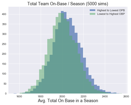
First thing we’ll look at is total number of times that a batter reached base in a season, for each simulation, for the bottom-up (green) and top-down (blue) lineups.
As you’d expect, on average, lineups where the better batters come first and thus have more opportunities to bat, get on base more often.
td_sim['box'][1]
plt.hist(td_total_hits, 'scott', alpha = 0.7)
plt.hist(bu_total_hits, 'scott', alpha = 0.5)
plt.title("Total Team On-Base / Season (5000 sims)", fontsize=16)
plt.xlabel("Avg. Total On Base in a Season", fontsize=16)
labels= ["Highest to Lowest OPB","Lowest to Highest OBP"]
plt.legend(labels)
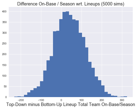
Howver, plotting the difference we find the advantage is not huge, with the peaks of the distributions off by less than 40. Or an extra on-base every 4 games.
td_sim['box'][1]
plt.hist(td_total_hits - bu_total_hits, 'scott')
plt.title("Difference On-Base / Season wrt. Lineups (5000 sims)", fontsize=16)
plt.xlabel("Top-Down minus Bottom-Up Lineup Total Team On-Base/Season", fontsize=16)
labels= ["Highest to Lowest OPB","Lowest to Highest OBP"]
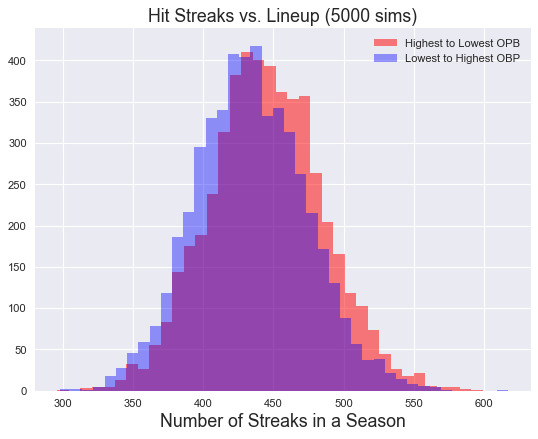
What about streaks?
Plotting number of streaks in a season we find similar behavoir favoring top-down OBPs.
fig= plt.figure()
fig.patch.set_alpha(0.5)
plt.hist(td_streak_count, 'scott', alpha = 0.5, color = 'r')
plt.hist(bu_streak_count, 'scott',alpha = 0.4, color = 'b')
plt.title("Hit Streaks vs. Lineup (5000 sims)", fontsize=16)
plt.xlabel("Number of Streaks in a Season", fontsize=16)
plt.legend(labels)
labels= ["Highest to Lowest OPB","Lowest to Highest OBP"]
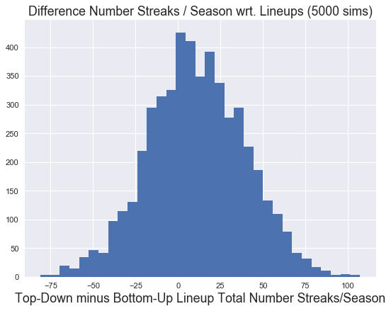
And that the difference in total number of streaks peaks at around 10.
td_sim['box'][1]
plt.hist(td_streak_count - bu_streak_count, 'scott')
plt.title("Difference Number Streaks / Season wrt. Lineups (5000 sims)", fontsize=16)
plt.xlabel("Top-Down minus Bottom-Up Lineup Total Number Streaks/Season", fontsize=16)
labels= ["Highest to Lowest OPB","Lowest to Highest OBP"]
Conclusion
Batting order is not irrelevant, but as for reaching base more often, or for promoting hits in clusters, simple simulations indicate a small effect over a full season.
But this is need not be the end of the story. This simulation does not take into account any covariances in the batting order; i.e., does the outcome of an at-bat effect the batter in front or behind them in the order? And here at-bats are either outs or walks, what if more options are included?
This is the kind of simulation that gets built in stages. More to come.